Fri, 27.04. Decision Making

I had gotten up very early to make an all-day recording with our Davis346 silicon retina of "life in the hotel bar".  After fiddling around with various  filters like BackgroundActivityFilter, DvsBiasController, and DavisAutoShooter, I crossed my fingers and set the whole thing going, recording onto  an external hard disk, and headed for breakfast. 

On the way I passed the early yoga group and admired the view. 

Gradually people appeared for breakfast, like Greg Cohen and Barry Richmond.

At 9am we started the morning discussion, about decision making.  This session was organized by a large cast of people including Yulia Sandamirskaya, Mathew Diamond, Barry Richmond, Paolo Del Giudice, and Valerio Mante. This group was clearly dominated by biologists, with some cognitive robotics, physics and computational neuroscience also included.

The focus was on understanding how brains come to decisions to take actions and what neural circuits express and are involved in these these discrete choice events, where the animal has weighed evidence and finally decided to take one action from a set of discrete alternative choices.

Valerio's working definition of a decision is a choice from a set of alternative choices.
The decision process gets input from perception, motivation, memory, value payoffs, etc to finally result in the decision. How do we characterize a model in animals and people?
The space is placed on space with 2 axes. Following David Marr, the vertical is concrete "neural" to "abstract". Other axis is the nature of representation used, from "spatialized" to "distributed". To be more concrete, there is a box, with stuff coming in and decision coming out.

One example is a the coherent colored red/green moving dots moving horizontally.  The subject has a context, e.g. motion or color. There is some evidence signal for each percept, e.g. motion direction or color. One way to solve this is to multiply one by context signal and the other by (1-context) and integrate the result over time. The signals are noisy because the stimuli are barely perceivable. If the subject is under time pressure, then they must make a decision. If they do this by setting a vertical bound and taking the decision when they reach a bound, then if the bounds are moved out, noise is reduced but latency is increased. It also explains confidence: If the decision takes longer, then confidence in choice is reduced since the subject understands the signal is noisier.  This description is quite abstract but useful to describe behavior and is also mathematically ideal based on certain assumptions on noise, constrained by some speed-accuracy tradeoff.

Also, many "neural correlates" of such evidence signals have been observed experimentally for decades.

Paulo del Guidice pointed out that such signals have been observed. No doubt such single neuron signals have been observed. But there is still some controversy about whether this is also true for population codes.

Barry Richmond pointed out that some people have tried to interfere with this signal without success on perturbing behavior. But others find for example if area MT is stimulated electrically it can bias the choices.

Such a model can be implemented neurally using a circuit with 3 populations of units that are connected so that two of them are mutually inhibited by a third. Each excitatory population excites itself to maintain its state. You need NMDA, AMPA, GABA, fast and  time constants, etc, which exhibits this choice behavior with realistic biophysics and temporal dynamics. But there is another level in between, which is to ask an artificial neural network, a vanilla RNN with recurrent connections and dynamics and linear readout. There is an input to set context (color or motion), and this network can be trained by backpropation through time (BPTT) to solve the problem.

What you get are two line attractors. Movement along the line attracctor corresponds to evidence. Pulses e.g. of motion move along the attractor, like integration. If the context input is changed to the other task, then the network moves to the other attractor and integrates along it. Valerio pointed out that it is remarkable that this evidence integration emerges from this collective behavior, and that it is impossible to separate out the components contributing to this collective behavior.  Actually these line attractors are a series of Hopf fixed points that generate stable points.

If the RNN connections are examined before and after training, then it is observed that the recurrent connectivity hardly changes. There is always a solution nearby that implements these line attractor dynamics.

Valerio believes one crucial test is to perturb the network and see if the responses correspond to theory. These experiments are ongoing.
The final point is that if you train a different task, e.g.  reaching, then you get very similar dynamics. He is a bit worried that such theoretical results indicate we might be missing something simple that is related to the structure of the problem that is posed and the architecture (RNN) that can demonstrate it. Do we really learn something?  Maybe from the regularizers that sometimes need to be applied.

At 10am,  Paulo del Guidice continued the discussion. He started off pointing out that he would be in the lower right corner, closer to neural. He talked about a model of attractor dynamics and to see if evidence of these dynamics are really observed.  The experiment is a reaching decision task with a stop signal that indicates that the reach should be aborted.  It is a called a countermand study, and was studied greatly in eye movements. Paulo's colleagues measured from dorsal premotor cortex the resulting signals from a monkey centering their finger on a center spot. The go signal is the disappearance of the spot. There is a reaction time, a movement, and then a reward. The monkey is about 100% correct. But, about 1/3 of trials are "stop" trials. After the spot disappears, after a certain delay called stop signal delay,  the center spot lights up again. If the monkey is able to inhibit the reach, it is rewarded. 

One the reactiion times are characterized, then the stop trial delays are chosen to create errors about 50% of the time. 

All this was known. But recent recordings from Stefano ?? with 96 electrode arrays provides new data. If the responses are plotted as channel activity vs time, then it is possible to try to reduce dimensionality to see if there are lower dimensional clusters. Paulo's group used clustering to compress and simplify in time. They used "density based clustering" derived from mean shift clustering (also used for object tracking from DVS event camera output). Then the result is a symbolic sequence of such clusters, e.g. AABC.  This clustering can be interpreted as climbing some energy landscape. But this is only a metaphor that might have nothing  to do with the neural dynamics.

Paulo then drew this interesting diagram:

Each row represents a trial. They are sorted by reaction time. The symbolic clusters make transitions according to the color hatching, but a key point is that there is a transition to a special set of clusters at some time before the movement start (red hatching). All these trials were from non-stop trials.

Things change for stop trials, shown as the lower sketch.  For unsuccessful stop trials, the monkey seems to be at the end of what is probably the motor planning period and cannot inhibit the plan.  

The analysis shows close to 90% correct on single trials to predict correct and incorrect responses based on the sequence of symbolic labels. 

Paulo concluded with a challenge to face reality. He asked, does attractor dynamics really have a useful role? For  example, what about inter-trial variability? He drew the diagram below

The usual interpretation is that at the minima the attractor is converging on a point attractor at the point of decision. But it could be that the system is moving along a valley rather than collapsing on point attractor. The result of measuring whether the system moves along gradients indicates that it does move toward attractors, but to summarize, their results indicate that the system is moving into channel dynamics rather than point attractors, indicating that the system is constantly still moving, not falling to stationary fixed points. They believe that this kind of analysis leads to simpler and more obvious interpretations of decision dynamics.

After the coffee break, Barry Richmond (NIH) continued to talk about decision making. He summarized slightly facetiously that there have been decades of results claiming to have found the "seat of the soul", and that he would not do this. Instead, he drew a diagram of primate brain to show important areas involved in decision making.

Information flowing along lateral temporal cortex is about identity, but medial temporal cortex flow is about value. They combine in frontal cortex. They all also are connected to striatum.  
He then described the task invented by Bob Wirz where monkey's are trained to fixate on a spot and to release a handle when the red spot turns green. If the monkey lets go, then it gets a drop of juice. l this task to macaque monkey takes about 3 weeks. After this task is trained, then one more refinement is added, where a value is added by 1 to 3 drops of juice. But to get 2 drops they have to wait 3 seconds, and for 3 drops, 7 seconds. They don't like to wait. Each type of trial has a different visual cue like some bar patterns.

Do they get a continuous scale of values? I.e. can they weigh reward with delay? If you plot refusals (early releases) vs drop size, you observe that monkeys clearly can account for reward/delay. And the "discounted reward" and probability of accepting each offer (trial) are related by very predictable functional relations in this sketch.

But if you ablate rhinal cortex, then the monkeys can no longer do this weighing. 

Rodney asked, is any behavior change observed after this ablation? 

Barry responded that there are no very obvious changes, except for cingulate. Rhesus monkeys are more aggressive and thus easier to train since they are not afraid of exploring.   These rhesus become more passive. With new tools, reversible chemical inhibition can be done as for optogenetic tools, but chemical. With the reversible lesion, lesioning orbitofrontal cortex deletes this value weighing. Lesioning striatum has similar effect. These new tools allow distinguishing the roles of medial temporal and orbitofrontal contributions to weighing value.


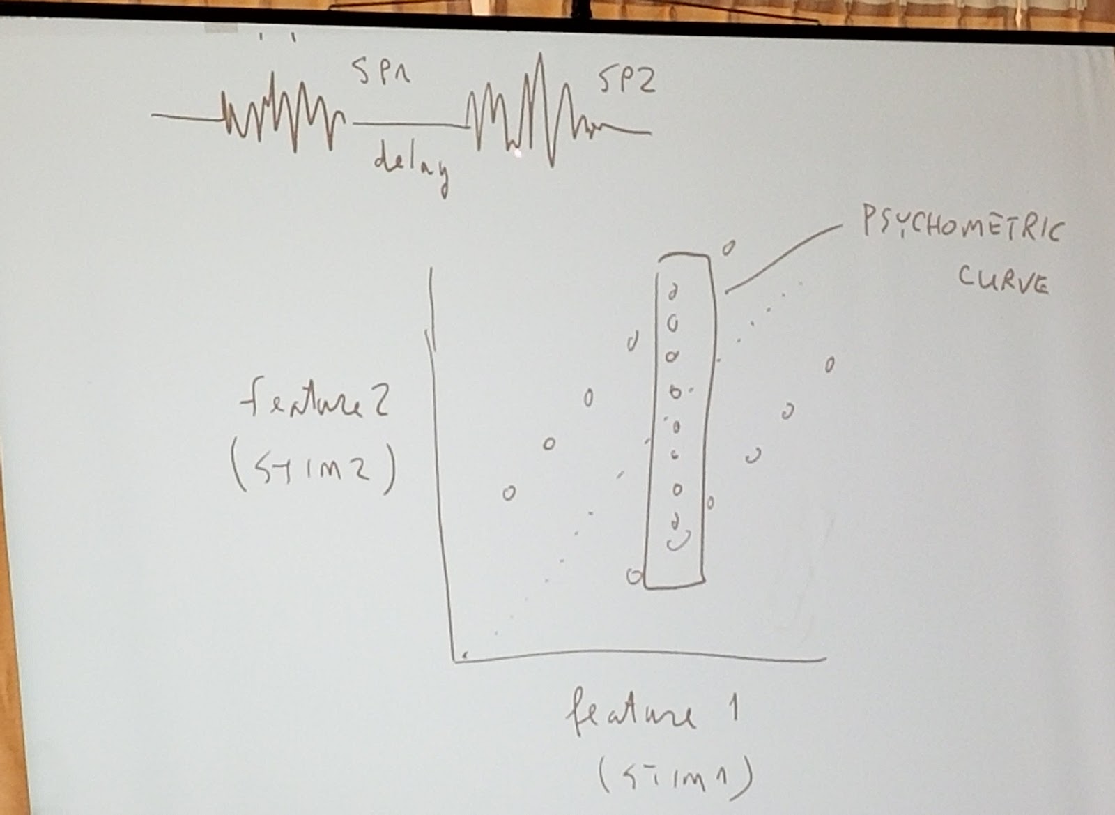
Matthew Diamond continued by describing work from Fassihi and Toso and his group. The rat pokes nose into chamber (or human puts finger in contact with buzzer) and has to distinguish vibration pattern generated from sample Gaussian velocity that is bandlimited to about 120Hz. The parameters are amplitude (speed=SP in sketch) and duration of vibration. There are two stimuli, with T1 and SP1, and T2 and SP2. The subject has to either pay attention to amplitude or duration. They have to see if second stimulus is bigger or less than first, for the specified duration or speed amplitude.

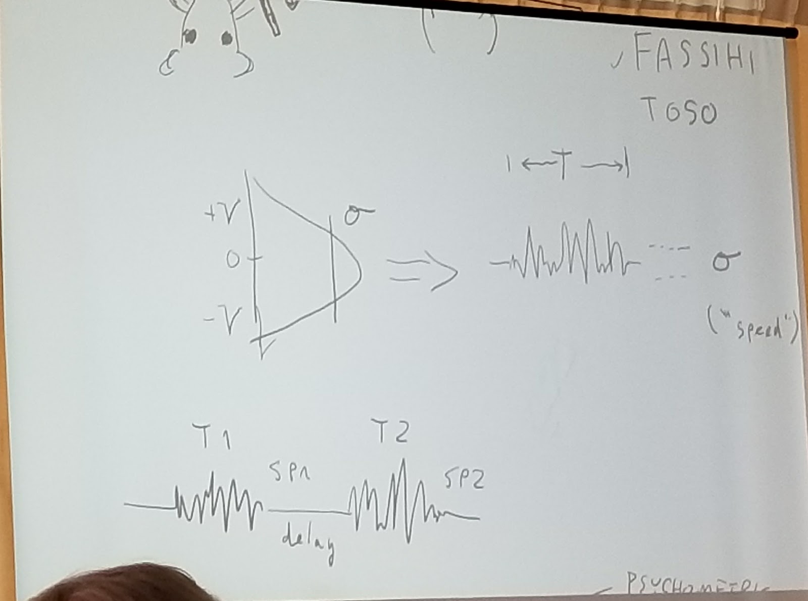
The result is a typical  psychrometric curve plotted in this sketch, for both speed amplitude and duration. 

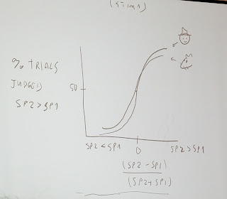
But using the set of stimulis for speed and duration in the sketch below, the longer vibrations feel stronger and the strong vibrations feel longer, as shown by shifts of the psychrometric curves.

It suggests that there is an internal representation of evidence that  is consistent with Valerio's earlier discussion. This confounding of the stimuli dimensions is not optimal, suggesting a projection that is as good as possible given the sensory integration.

Finally, Yulia showed how an entire hierarchy of decisions can be built from a neural circuit using interconnected units wired up as illustrated in the sketch below.

The discussion ran well into lunchtime and so there was a break for lunch and the discussion continued at 4pm.